Part A: Adaptive time-stepping

So far, all our steps had the same size. For many problems this is wasteful: the solution changes quickly at some times and slowly at others, and a fixed step size has to be small enough for the fastest phase. pySDC can choose the step size on the fly with the Adaptivity convergence controller. We try it on the van der Pol oscillator

\[ u'' - \mu (1 - u^2) u' + u = 0 \]

with \(\mu = 5\), written as a system for \(u\) and \(u'\) in vanderpol. In \([0, 10]\), its solution creeps along, jumps once, and creeps along again. We solve it with implicit SDC and exactly 4 iterations per step. The function below does one run, with the fixed step size dt or, if a tolerance e_tol is given, adaptively, starting with dt.

import matplotlib.pyplot as plt
import numpy as np

from pySDC.helpers.stats_helper import get_sorted
from pySDC.implementations.controller_classes.controller_nonMPI import controller_nonMPI
from pySDC.implementations.convergence_controller_classes.adaptivity import Adaptivity
from pySDC.implementations.hooks.log_solution import LogSolution
from pySDC.implementations.hooks.log_work import LogWork
from pySDC.implementations.problem_classes.Van_der_Pol_implicit import vanderpol
from pySDC.implementations.sweeper_classes.generic_implicit import generic_implicit

mu = 5.0
Tend = 10.0


def run_vdp(dt, e_tol=None):
    description = {
        'problem_class': vanderpol,
        'problem_params': {'mu': mu, 'newton_tol': 1e-9, 'relative_tolerance': True},
        'sweeper_class': generic_implicit,
        'sweeper_params': {'quad_type': 'RADAU-RIGHT', 'num_nodes': 3, 'QI': 'LU'},
        'level_params': {'dt': dt},  # no restol: every step does maxiter iterations
        'step_params': {'maxiter': 4},
    }
    if e_tol is not None:
        description['convergence_controllers'] = {Adaptivity: {'e_tol': e_tol}}

    controller_params = {
        'logger_level': 30,
        'mssdc_jac': False,  # Adaptivity refuses the (default) Jacobi mode of multi-step SDC
        'hook_class': [LogSolution, LogWork],
    }
    controller = controller_nonMPI(num_procs=1, controller_params=controller_params, description=description)
    P = controller.MS[0].levels[0].prob
    return controller.run(u0=P.u_exact(0.0), t0=0.0, Tend=Tend)


# reference solution at Tend, computed once with scipy's solve_ivp at a tight tolerance
u_ref = vanderpol(mu=mu).u_exact(Tend)


def summary(uend, stats):
    """Accepted steps, restarts, the work of all steps, restarted ones included, and the error at the end."""
    return {
        't_end': get_sorted(stats, type='u', recomputed=False)[-1][0],
        'steps': len(get_sorted(stats, type='niter', recomputed=False)),
        'restarts': sum(me[1] for me in get_sorted(stats, type='restart')),
        'iterations': sum(me[1] for me in get_sorted(stats, type='niter')),
        'rhs': sum(me[1] for me in get_sorted(stats, type='work_rhs')),
        'newton': sum(me[1] for me in get_sorted(stats, type='work_newton')),
        'error': abs(uend - u_ref),
    }


def show(name, me):
    print(
        f"{name:>12}: {me['steps']:4d} steps, {me['restarts']:3d} restarts, {me['iterations']:5d} iterations, "
        f"{me['rhs']:6d} right-hand sides, {me['newton']:5d} Newton iterations, error {me['error']:.2e}"
    )

LogSolution records the solution after each step and LogWork the increments of the problem’s work counters, here of right-hand side evaluations and Newton iterations. The error is measured against a reference solution from scipy.

An adaptive run

All it takes is the Adaptivity convergence controller with a tolerance e_tol for the local error. We start with a small step and let it grow:

e_tol = 2e-5
uend, stats = run_vdp(dt=1e-2, e_tol=e_tol)
adaptive = summary(uend, stats)
show('adaptive', adaptive)

    adaptive:   77 steps,  27 restarts,   416 iterations,   1664 right-hand sides,  2072 Newton iterations, error 7.23e-06

Adaptivity adds the hooks it needs itself: LogStepSize records the step size as dt, and the error estimate it relies on comes with LogEmbeddedErrorEstimate. The restarts are recorded by LogRestarts, which comes with the restarting that controller_nonMPI always has. When a step is restarted, its values stay in the statistics; recomputed=False in get_sorted leaves them out and keeps only the accepted steps.

u = get_sorted(stats, type='u', recomputed=False)
dt = get_sorted(stats, type='dt', recomputed=False)
e_em = get_sorted(stats, type='error_embedded_estimate', recomputed=False)
restart_times = [t for t, restarted in get_sorted(stats, type='restart') if restarted]

ratio = np.array([e for _, e in e_em]) / e_tol
print(f'estimate / e_tol of the accepted steps: median {np.median(ratio):.2f}, max {ratio.max():.2f}')

estimate / e_tol of the accepted steps: median 0.48, max 0.96

Show code cell source

Hide code cell source

fig, axs = plt.subplots(3, 1, figsize=(8, 6), sharex=True, constrained_layout=True)
axs[0].plot([t for t, _ in u], [v[0] for _, v in u], label="$u$")
axs[0].plot([t for t, _ in u], [v[1] for _, v in u], label="$u'$")
axs[0].legend(frameon=False)
axs[0].set_ylabel('solution')
axs[1].semilogy([t for t, _ in dt], [v for _, v in dt], '.-', color='black')
for t in restart_times:
    axs[1].axvline(t, color='grey', ls=':', lw=0.8)
axs[1].set_ylabel(r'$\Delta t$ (dotted: restarts)')
axs[2].semilogy([t for t, _ in e_em], [v for _, v in e_em], '.', color='magenta', label='embedded estimate')
axs[2].axhline(e_tol, color='black', ls='--', label='e_tol')
axs[2].legend(frameon=False)
axs[2].set_ylabel('local error')
axs[2].set_xlabel('time')
for ax in axs:
    ax.grid(alpha=0.3)

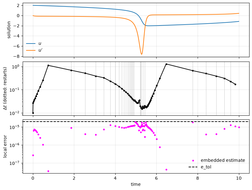
The step size follows the solution: it grows from the initial \(0.01\) to about \(1\) within the first time unit, shrinks as the jump approaches, is smallest (\(0.015\)) at \(t \approx 5.3\), where \(u\) changes fastest (\(u'\) reaches \(-7.6\)), and grows again to its largest value (\(1.28\)) after the jump. The estimates of the accepted steps stay below e_tol, and all but 5 of the 77 above a tenth of it: their median is \(0.48\) e_tol.

How it works

• Error estimate. Each iteration raises the order of SDC by one, so the solution of the next-to-last iteration is a lower order approximation than that of the last one. EstimateEmbeddedError takes the difference of the two at the end of the step as an estimate of the local error of the lower order one: the embedded error estimate.

• New step size. After the last iteration, the next step size is \(\Delta t_\mathrm{new} = \beta \, \Delta t \, (\epsilon_\mathrm{tol} / \epsilon)^{1/k}\), with the estimate \(\epsilon\), the tolerance \(\epsilon_\mathrm{tol}\) (e_tol), the safety factor \(\beta\) (beta, 0.9 by default), and \(k\) the number of iterations, which the code uses as the order of the estimate. Hence, all steps must do the same number of iterations: Adaptivity refuses a residual tolerance restol of zero or more.

• Restarts. If \(\epsilon\) is not below \(\epsilon_\mathrm{tol}\), the step is not accepted but restarted with \(\Delta t_\mathrm{new}\), which is then smaller than \(\Delta t\). A step that still fails after 10 restarts in a row stops the run with a ConvergenceError (parameters max_restarts and crash_after_max_restarts of BasicRestarting).

The rule proposes the next step as if the error behaves there as in the current one. Where the error grows from step to step, as on the way to the jump, the proposal is too large and the step is restarted. That is where most of the restarts are: each of them redid one step, and none had to redo a step twice.

A comparison with fixed steps

The same SDC with fixed step sizes, halving them until the error matches that of the adaptive run:

dts_fixed = [1 / 8, 1 / 16, 1 / 32]
fixed = [summary(*run_vdp(dt=me)) for me in dts_fixed]
for dt_fixed, me in zip(dts_fixed, fixed, strict=True):
    show(f'dt = 1/{round(1 / dt_fixed)}', me)
show('adaptive', adaptive)

    dt = 1/8:   80 steps,   0 restarts,   320 iterations,   1280 right-hand sides,  1438 Newton iterations, error 6.84e-04
   dt = 1/16:  160 steps,   0 restarts,   640 iterations,   2560 right-hand sides,  2617 Newton iterations, error 9.33e-05
   dt = 1/32:  320 steps,   0 restarts,  1280 iterations,   5120 right-hand sides,  4768 Newton iterations, error 7.31e-06
    adaptive:   77 steps,  27 restarts,   416 iterations,   1664 right-hand sides,  2072 Newton iterations, error 7.23e-06

Show code cell source

Hide code cell source

fig, ax = plt.subplots(figsize=(6, 3.5), constrained_layout=True)
ax.loglog([me['newton'] for me in fixed], [me['error'] for me in fixed], 'o-', label='fixed step size')
for dt_fixed, me in zip(dts_fixed, fixed, strict=True):
    ax.annotate(f' 1/{round(1 / dt_fixed)}', (me['newton'], me['error']))
ax.loglog(adaptive['newton'], adaptive['error'], '*', ms=12, label='adaptive')
ax.set_xlabel('Newton iterations')
ax.set_ylabel('error at the end')
ax.legend(frameon=False)
ax.grid(alpha=0.3)

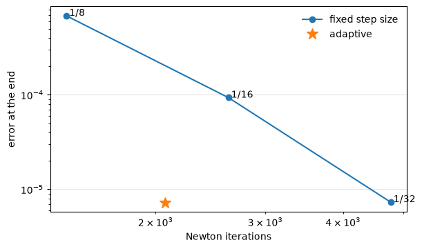
With \(\Delta t = 1/32\), the error is the same as with adaptivity, \(7.3 \cdot 10^{-6}\) against \(7.2 \cdot 10^{-6}\). For that, the fixed steps need 320 steps, 1280 iterations, 5120 right-hand side evaluations and 4768 Newton iterations. The adaptive run gets there with 77 steps plus 27 restarts, 416 iterations, 1664 right-hand side evaluations and 2072 Newton iterations: about a third of the iterations, although a quarter of them went into restarted steps, and less than half the Newton iterations.

Important things to note

• e_tol bounds the estimated local error of each step, not the error at the end. Here, a local tolerance of \(2 \cdot 10^{-5}\) gave an error of \(7.2 \cdot 10^{-6}\) at the end, but the relation depends on the problem.

• The step size can be limited with the parameters dt_min and dt_max of Adaptivity, which pass them on to the StepSizeLimiter convergence controller.

• With avoid_restarts, Adaptivity estimates from the contraction of the iteration how many more iterations would reach the tolerance, and continues iterating instead of restarting if they are few enough.

The checks the tests run:

assert all(me['t_end'] == Tend for me in [adaptive] + fixed), 'ERROR: not all runs reached Tend'
assert ratio.max() < 1, f'ERROR: an accepted step has an estimate above the tolerance: {ratio.max()}'
assert adaptive['restarts'] > 0, 'ERROR: expected restarts in the adaptive run'
assert (
    adaptive['error'] < 1.1 * fixed[-1]['error']
), f"ERROR: adaptive run is less accurate than dt=1/32: {adaptive['error']:.2e} vs. {fixed[-1]['error']:.2e}"
assert (
    adaptive['iterations'] < fixed[-1]['iterations'] / 2
), f"ERROR: adaptive run needs too many iterations: {adaptive['iterations']} vs. {fixed[-1]['iterations']}"
assert (
    adaptive['newton'] < fixed[-1]['newton'] / 2
), f"ERROR: adaptive run needs too many Newton iterations: {adaptive['newton']} vs. {fixed[-1]['newton']}"