Part C: Collocation problem setup

Now time enters. Written in integral form, the heat equation from Part A reads

\[ u(t) = u_0 + \int_{t_0}^{t} A\, u(s)\, ds , \]

with \(A\) the finite-difference Laplacian (times \(\nu\)). Collocation replaces the integral by a quadrature rule on \(M\) nodes \(t_0 + \tau_m \Delta t\) inside one time step, and demands that the equation holds exactly at these nodes. Whatever the equation, this collocation problem of one time step is what the methods in pySDC solve; the heat equation is just the example here.

import matplotlib.pyplot as plt
import numpy as np
import scipy.sparse as sp

from pySDC.core.collocation import CollBase
from pySDC.implementations.problem_classes.HeatEquation_ND_FD import heatNd_unforced

prob = heatNd_unforced(
    nvars=1023,  # number of degrees of freedom
    nu=0.1,  # diffusion coefficient
    freq=4,  # frequency for the test value
    bc='dirichlet-zero',  # boundary conditions
)

Nodes and the collocation matrix

CollBase provides the quadrature: here three Gauss-Radau nodes, whose last node is the right end of the interval. node_type picks the family of nodes (Legendre here), quad_type which ends of the interval are nodes themselves: none ('GAUSS'), one ('RADAU-LEFT', 'RADAU-RIGHT') or both ('LOBATTO').

# instantiate collocation class, relative to the time interval [0,1]
coll = CollBase(num_nodes=3, tleft=0, tright=1, node_type='LEGENDRE', quad_type='RADAU-RIGHT')

with np.printoptions(precision=4, suppress=True):
    print('nodes tau_m:', coll.nodes)
    print('Q =')
    print(coll.Qmat[1:, 1:])

nodes tau_m: [0.1551 0.6449 1.    ]
Q =
[[ 0.1968 -0.0655  0.0238]
 [ 0.3944  0.2921 -0.0415]
 [ 0.3764  0.5125  0.1111]]

Row \(m\) of the matrix \(Q = (q_{mj})\) holds the quadrature weights for the integral from \(0\) to \(\tau_m\). Its first row and column in coll.Qmat belong to the initial value and are dropped. Both are relative to \([0, 1]\): multiply by \(\Delta t\) for a real time step. The collocation problem for the values \(u_m \approx u(t_0 + \tau_m \Delta t)\) is then

\[ u_m = u_0 + \Delta t \sum_{j=1}^{M} q_{mj} A u_j \quad\Longleftrightarrow\quad (I - \Delta t\, Q \otimes A)\, \vec u = \vec u_0 . \]

Solving it directly

The problem is linear, so we can assemble the Kronecker product and hand it to a sparse direct solver. Since the last Radau node is the end of the step, the last block of the solution is \(u(\Delta t)\), which we compare with the exact solution.

def solve_collocation_problem(prob, coll, dt):
    """
    Routine to build and solve the linear collocation problem

    Args:
        prob: a problem instance
        coll: a collocation instance
        dt: time-step size

    Return:
        the analytic error of the solved collocation problem
    """

    # shrink collocation matrix: first line and column deals with initial value, not needed here
    Q = coll.Qmat[1:, 1:]

    # build system matrix M of collocation problem
    M = sp.eye(prob.nvars[0] * coll.num_nodes) - dt * sp.kron(Q, prob.A)

    # get initial value at t0 = 0
    u0 = prob.u_exact(t=0)
    # fill in u0-vector as right-hand side for the collocation problem
    u0_coll = np.kron(np.ones(coll.num_nodes), u0)
    # get exact solution at Tend = dt
    uend = prob.u_exact(t=dt)

    # solve collocation problem directly
    u_coll = sp.linalg.spsolve(M, u0_coll)

    # compute error
    err = np.linalg.norm(u_coll[-prob.nvars[0] :] - uend, np.inf)

    return err


# set time-step size (warning: the collocation matrices are relative to [0,1], see above)
dt = 0.1
err = solve_collocation_problem(prob=prob, coll=coll, dt=dt)
print(f'Error of the collocation problem: {err:8.6e}')

Error of the collocation problem: 3.803471e-04

Why pySDC does not do it like this

The system couples all nodes: every block of \(Q \otimes A\) is a scaled copy of \(A\). For a small mesh the structure is easy to see:

Show code cell source

Hide code cell source

small = heatNd_unforced(nvars=15, nu=0.1, freq=4, bc='dirichlet-zero')
M_small = sp.eye(15 * coll.num_nodes) - dt * sp.kron(coll.Qmat[1:, 1:], small.A)
fig, ax = plt.subplots(figsize=(3.5, 3.5))
ax.spy(M_small, markersize=3)
ax.set_title(r'$I - \Delta t\, Q \otimes A$, 15 unknowns, $M = 3$', fontsize=10)
fig.tight_layout()

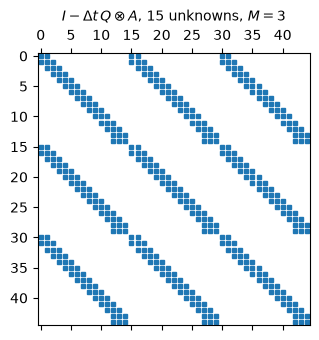
That is \(M\) times more unknowns than a single implicit Euler step, fully coupled. Fine for a 1D heat equation, hopeless for a 3D problem with a nonlinear right-hand side. The rest of pySDC therefore never assembles this matrix: it keeps space and time separate and solves the collocation problem iteratively with SDC, starting in Step 2.

Important things to note

• The collocation matrix Q is and will always be relative to \([0, 1]\). Use dt to scale it.

• u_exact gives the solution at any time. Give your own problem classes either an exact solution or an initial condition routine.

• This is where the fun with parameters starts: how many unknowns in space, how large a dt, how high a frequency? Try some and watch the error.

The check the tests run:

assert err <= 4e-04, f"ERROR: did not get collocation error as expected, got {err}"