Step-1: A first spatial problem

In this step, we create a spatial problem and play with it a little bit. No SDC, no multi-level here so far.

Part A: Spatial problem setup

We start as simple as possible by creating a first, very simple problem using one of the problem_classes, namely HeatEquation_1D_FD. This basically consists only of the matrix A, which represents a finite difference discretization of the 1D Laplacian. This is tested for one particular example.

Important things to note:

• Many (most) parameters for pySDC are passed using dictionaries

• Data types are encapsulated: the real values are stored in values, meta-information can be stored separately in the data structure

• A quick peak into HeatEquation_1D_FD reveals that the init and the params.nvars attribute contain the same values (namely nvars). Yet, sometimes one or the other is used here (and throughout the code). The reason is this: the data structure (mesh in this case) needs some form of standard initialization. For this, pySDC uses the init attribute each problem class has. In our simple example, this is he same as nvars, but e.g. for Finite Elements, the function space is stored in the init attribute. Thus, whenever a data type is created, use init, otherwise do whatever looks nice.

• We happily pass classes around so that they can be used to instantiate things within subroutines

Full code: pySDC/tutorial/step_1/A_spatial_problem_setup.py

import numpy as np
from pathlib import Path

from pySDC.implementations.problem_classes.HeatEquation_ND_FD import heatNd_unforced


def main():
    """
    A simple test program to set up a spatial problem and play with it
    """
    # instantiate problem
    prob = heatNd_unforced(
        nvars=1023,  # number of degrees of freedom
        nu=0.1,  # diffusion coefficient
        freq=4,  # frequency for the test value
        bc='dirichlet-zero',  # boundary conditions
    )

    # run accuracy test, get error back
    err = run_accuracy_check(prob)

    Path("data").mkdir(parents=True, exist_ok=True)
    f = open('data/step_1_A_out.txt', 'w')
    out = 'Error of the spatial accuracy test: %8.6e' % err
    f.write(out)
    print(out)
    f.close()

    assert err <= 2e-04, "ERROR: the spatial accuracy is higher than expected, got %s" % err


def run_accuracy_check(prob):
    """
    Routine to check the error of the Laplacian vs. its FD discretization

    Args:
        prob: a problem instance

    Returns:
        the error between the analytic Laplacian and the computed one of a given function
    """

    # create x values, use only inner points
    xvalues = np.array([(i + 1) * prob.dx for i in range(prob.nvars[0])])

    # create a mesh instance and fill it with a sine wave
    u = prob.dtype_u(init=prob.init)
    u[:] = np.sin(np.pi * prob.freq[0] * xvalues)

    # create a mesh instance and fill it with the Laplacian of the sine wave
    u_lap = prob.dtype_u(init=prob.init)
    u_lap[:] = -((np.pi * prob.freq[0]) ** 2) * prob.nu * np.sin(np.pi * prob.freq[0] * xvalues)

    # compare analytic and computed solution using the eval_f routine of the problem class
    err = abs(prob.eval_f(u, 0) - u_lap)

    return err


if __name__ == "__main__":
    main()

Results:

Error of the spatial accuracy test: 1.981783e-04

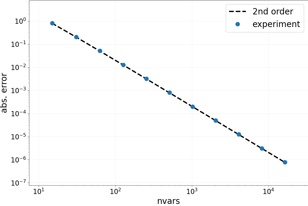
Part B: Spatial accuracy check

We now do a more thorough test of the accuracy of the spatial discretization. We loop over a set of nvars, compute the Laplacian of our test vector and look at the error. Then, the order of accuracy in space is checked by looking at the numbers and by looking at “points on a line”.

Important things to note:

• You better test your operators.. use nvars > 2**16 and things will break!

• Add your results into a dictionary for later usage. Use IDs to find the data! Also, use headers to store meta-information.

Full code: pySDC/tutorial/step_1/B_spatial_accuracy_check.py

from pathlib import Path
import matplotlib

matplotlib.use('Agg')

from collections import namedtuple
import matplotlib.pylab as plt
import numpy as np
import os.path

from pySDC.implementations.datatype_classes.mesh import mesh
from pySDC.implementations.problem_classes.HeatEquation_ND_FD import heatNd_unforced

# setup id for gathering the results (will sort by nvars)
ID = namedtuple('ID', 'nvars')


def main():
    """
    A simple test program to check order of accuracy in space for a simple test problem
    """

    # initialize problem parameters
    problem_params = dict()
    problem_params['nu'] = 0.1  # diffusion coefficient
    problem_params['freq'] = 4  # frequency for the test value
    problem_params['bc'] = 'dirichlet-zero'  # boundary conditions

    # create list of nvars to do the accuracy test with
    nvars_list = [2**p - 1 for p in range(4, 15)]

    # run accuracy test for all nvars
    results = run_accuracy_check(nvars_list=nvars_list, problem_params=problem_params)

    # compute order of accuracy
    order = get_accuracy_order(results)

    Path("data").mkdir(parents=True, exist_ok=True)
    f = open('data/step_1_B_out.txt', 'w')
    for l in range(len(order)):
        out = 'Expected order: %2i -- Computed order %4.3f' % (2, order[l])
        f.write(out + '\n')
        print(out)
    f.close()

    # visualize results
    plot_accuracy(results)

    assert os.path.isfile('data/step_1_accuracy_test_space.png'), 'ERROR: plotting did not create file'

    assert all(np.isclose(order, 2, rtol=0.06)), "ERROR: spatial order of accuracy is not as expected, got %s" % order


def run_accuracy_check(nvars_list, problem_params):
    """
    Routine to check the error of the Laplacian vs. its FD discretization

    Args:
        nvars_list: list of nvars to do the testing with
        problem_params: dictionary containing the problem-dependent parameters

    Returns:
        a dictionary containing the errors and a header (with nvars_list)
    """

    results = {}
    # loop over all nvars
    for nvars in nvars_list:
        # setup problem
        problem_params['nvars'] = nvars
        prob = heatNd_unforced(**problem_params)

        # create x values, use only inner points
        xvalues = np.array([(i + 1) * prob.dx for i in range(prob.nvars[0])])

        # create a mesh instance and fill it with a sine wave
        u = prob.u_exact(t=0)

        # create a mesh instance and fill it with the Laplacian of the sine wave
        u_lap = prob.dtype_u(init=prob.init)
        u_lap[:] = -((np.pi * prob.freq[0]) ** 2) * prob.nu * np.sin(np.pi * prob.freq[0] * xvalues)

        # compare analytic and computed solution using the eval_f routine of the problem class
        err = abs(prob.eval_f(u, 0) - u_lap)

        # get id for this nvars and put error into dictionary
        id = ID(nvars=nvars)
        results[id] = err

    # add nvars_list to dictionary for easier access later on
    results['nvars_list'] = nvars_list

    return results


def get_accuracy_order(results):
    """
    Routine to compute the order of accuracy in space

    Args:
        results: the dictionary containing the errors

    Returns:
        the list of orders
    """

    # retrieve the list of nvars from results
    assert 'nvars_list' in results, 'ERROR: expecting the list of nvars in the results dictionary'
    nvars_list = sorted(results['nvars_list'])

    order = []
    # loop over two consecutive errors/nvars pairs
    for i in range(1, len(nvars_list)):
        # get ids
        id = ID(nvars=nvars_list[i])
        id_prev = ID(nvars=nvars_list[i - 1])

        # compute order as log(prev_error/this_error)/log(this_nvars/old_nvars) <-- depends on the sorting of the list!
        tmp = np.log(results[id_prev] / results[id]) / np.log(nvars_list[i] / nvars_list[i - 1])
        order.append(tmp)

    return order


def plot_accuracy(results):
    """
    Routine to visualize the errors as well as the expected errors

    Args:
        results: the dictionary containing the errors
    """

    # retrieve the list of nvars from results
    assert 'nvars_list' in results, 'ERROR: expecting the list of nvars in the results dictionary'
    nvars_list = sorted(results['nvars_list'])

    # Set up plotting parameters
    params = {
        'legend.fontsize': 20,
        'figure.figsize': (12, 8),
        'axes.labelsize': 20,
        'axes.titlesize': 20,
        'xtick.labelsize': 16,
        'ytick.labelsize': 16,
        'lines.linewidth': 3,
    }
    plt.rcParams.update(params)

    # create new figure
    plt.figure()
    # take x-axis limits from nvars_list + some spacing left and right
    plt.xlim([min(nvars_list) / 2, max(nvars_list) * 2])
    plt.xlabel('nvars')
    plt.ylabel('abs. error')
    plt.grid()

    # get guide for the order of accuracy, i.e. the errors to expect
    # get error for first entry in nvars_list
    id = ID(nvars=nvars_list[0])
    base_error = results[id]
    # assemble optimal errors for 2nd order method and plot
    order_guide_space = [base_error / (2 ** (2 * i)) for i in range(0, len(nvars_list))]
    plt.loglog(nvars_list, order_guide_space, color='k', ls='--', label='2nd order')

    min_err = 1e99
    max_err = 0e00
    err_list = []
    # loop over nvars, get errors and find min/max error for y-axis limits
    for nvars in nvars_list:
        id = ID(nvars=nvars)
        err = results[id]
        min_err = min(err, min_err)
        max_err = max(err, max_err)
        err_list.append(err)
    plt.loglog(nvars_list, err_list, ls=' ', marker='o', markersize=10, label='experiment')

    # adjust y-axis limits, add legend
    plt.ylim([min_err / 10, max_err * 10])
    plt.legend(loc=1, ncol=1, numpoints=1)

    # save plot as PDF, beautify
    fname = 'data/step_1_accuracy_test_space.png'
    plt.savefig(fname, bbox_inches='tight')

    return None


if __name__ == "__main__":
    main()

Results:

Expected order:  2 -- Computed order 1.888
Expected order:  2 -- Computed order 1.949
Expected order:  2 -- Computed order 1.976
Expected order:  2 -- Computed order 1.988
Expected order:  2 -- Computed order 1.994
Expected order:  2 -- Computed order 1.997
Expected order:  2 -- Computed order 1.999
Expected order:  2 -- Computed order 1.999
Expected order:  2 -- Computed order 1.999
Expected order:  2 -- Computed order 1.982

Part C: Collocation problem setup

Here, we set up our first collocation problem using one of the collocation_classes, namely GaussRadau_Right. Using the spatial operator, we can build the collocation problem which in this case is linear. This fully coupled system is then solved directly and the error is compared to the exact solution.

Important things to note:

• The collocation matrix Q is and will be always relative to the temporal domain [0,1]. Use dt to scale it appropriately.

• Although convenient to analyze, the matrix formulation is not suited for larger (in space or time) computations. All remaining computations in pySDC are thus based on decoupling space and time operators (i.e. no Kronecker product).

• We can use the u_exact routine here to return the values at any given point in time. It is recommended to include either an initialization routine or the exact solution (if applicable) into the problem class.

• This is where the fun with parameters comes in: How many DOFs do we need in space? How large/small does dt have to be? What frequency in space is fine? …

Full code: pySDC/tutorial/step_1/C_collocation_problem_setup.py

import numpy as np
import scipy.sparse as sp
from pathlib import Path

from pySDC.core.Collocation import CollBase
from pySDC.implementations.problem_classes.HeatEquation_ND_FD import heatNd_unforced


def main():
    """
    A simple test program to create and solve a collocation problem directly
    """

    # instantiate problem
    prob = heatNd_unforced(
        nvars=1023,  # number of degrees of freedom
        nu=0.1,  # diffusion coefficient
        freq=4,  # frequency for the test value
        bc='dirichlet-zero',  # boundary conditions
    )

    # instantiate collocation class, relative to the time interval [0,1]
    coll = CollBase(num_nodes=3, tleft=0, tright=1, node_type='LEGENDRE', quad_type='RADAU-RIGHT')

    # set time-step size (warning: the collocation matrices are relative to [0,1], see above)
    dt = 0.1

    # solve collocation problem
    err = solve_collocation_problem(prob=prob, coll=coll, dt=dt)

    Path("data").mkdir(parents=True, exist_ok=True)
    f = open('data/step_1_C_out.txt', 'w')
    out = 'Error of the collocation problem: %8.6e' % err
    f.write(out + '\n')
    print(out)
    f.close()

    assert err <= 4e-04, "ERROR: did not get collocation error as expected, got %s" % err


def solve_collocation_problem(prob, coll, dt):
    """
    Routine to build and solve the linear collocation problem

    Args:
        prob: a problem instance
        coll: a collocation instance
        dt: time-step size

    Return:
        the analytic error of the solved collocation problem
    """

    # shrink collocation matrix: first line and column deals with initial value, not needed here
    Q = coll.Qmat[1:, 1:]

    # build system matrix M of collocation problem
    M = sp.eye(prob.nvars[0] * coll.num_nodes) - dt * sp.kron(Q, prob.A)

    # get initial value at t0 = 0
    u0 = prob.u_exact(t=0)
    # fill in u0-vector as right-hand side for the collocation problem
    u0_coll = np.kron(np.ones(coll.num_nodes), u0)
    # get exact solution at Tend = dt
    uend = prob.u_exact(t=dt)

    # solve collocation problem directly
    u_coll = sp.linalg.spsolve(M, u0_coll)

    # compute error
    err = np.linalg.norm(u_coll[-prob.nvars[0] :] - uend, np.inf)

    return err


if __name__ == "__main__":
    main()

Results:

Error of the collocation problem: 3.803471e-04

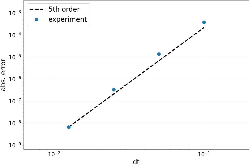
Part D: Collocation accuracy test

As for the spatial operator, we now test the accuracy in time. This time, we loop over a set of dt, compute the solution to the collocation problem and look at the error.

Important things to note:

• We take a large number of DOFs in space, since we need to beat 5th order in time with a 2nd order stencil in space.

• Orders of convergence are not as stable as for the space-only test. One of the problems of this example is that we are actually trying to compute 0 very, very thoroughly…

Full code: pySDC/tutorial/step_1/D_collocation_accuracy_check.py

from pathlib import Path
import matplotlib

matplotlib.use('Agg')

from collections import namedtuple
import matplotlib.pylab as plt
import numpy as np
import os.path
import scipy.sparse as sp

from pySDC.core.Collocation import CollBase
from pySDC.implementations.problem_classes.HeatEquation_ND_FD import heatNd_unforced

# setup id for gathering the results (will sort by dt)
ID = namedtuple('ID', 'dt')


def main():
    """
    A simple test program to compute the order of accuracy in time
    """

    # initialize problem parameters
    problem_params = {}
    problem_params['nu'] = 0.1  # diffusion coefficient
    problem_params['freq'] = 4  # frequency for the test value
    problem_params['nvars'] = 16383  # number of DOFs in space
    problem_params['bc'] = 'dirichlet-zero'  # boundary conditions

    # instantiate problem
    prob = heatNd_unforced(**problem_params)

    # instantiate collocation class, relative to the time interval [0,1]
    coll = CollBase(num_nodes=3, tleft=0, tright=1, node_type='LEGENDRE', quad_type='RADAU-RIGHT')

    # assemble list of dt
    dt_list = [0.1 / 2**p for p in range(0, 4)]

    # run accuracy test for all dt
    results = run_accuracy_check(prob=prob, coll=coll, dt_list=dt_list)

    # get order of accuracy
    order = get_accuracy_order(results)

    Path("data").mkdir(parents=True, exist_ok=True)
    f = open('data/step_1_D_out.txt', 'w')
    for l in range(len(order)):
        out = 'Expected order: %2i -- Computed order %4.3f' % (5, order[l])
        f.write(out + '\n')
        print(out)
    f.close()

    # visualize results
    plot_accuracy(results)

    assert os.path.isfile('data/step_1_accuracy_test_coll.png')

    assert all(np.isclose(order, 2 * coll.num_nodes - 1, rtol=0.4)), (
        "ERROR: did not get order of accuracy as expected, got %s" % order
    )


def run_accuracy_check(prob, coll, dt_list):
    """
    Routine to build and solve the linear collocation problem

    Args:
        prob: a problem instance
        coll: a collocation instance
        dt_list: list of time-step sizes

    Return:
        the analytic error of the solved collocation problem
    """

    results = {}
    # loop over all nvars
    for dt in dt_list:
        # shrink collocation matrix: first line and column deals with initial value, not needed here
        Q = coll.Qmat[1:, 1:]

        # build system matrix M of collocation problem
        M = sp.eye(prob.nvars[0] * coll.num_nodes) - dt * sp.kron(Q, prob.A)

        # get initial value at t0 = 0
        u0 = prob.u_exact(t=0)
        # fill in u0-vector as right-hand side for the collocation problem
        u0_coll = np.kron(np.ones(coll.num_nodes), u0)
        # get exact solution at Tend = dt
        uend = prob.u_exact(t=dt)

        # solve collocation problem directly
        u_coll = sp.linalg.spsolve(M, u0_coll)

        # compute error
        err = np.linalg.norm(u_coll[-prob.nvars[0] :] - uend, np.inf)
        # get id for this dt and store error in results
        id = ID(dt=dt)
        results[id] = err

    # add list of dt to results for easier access
    results['dt_list'] = dt_list
    return results


def get_accuracy_order(results):
    """
    Routine to compute the order of accuracy in time

    Args:
        results: the dictionary containing the errors

    Returns:
        the list of orders
    """

    # retrieve the list of dt from results
    assert 'dt_list' in results, 'ERROR: expecting the list of dt in the results dictionary'
    dt_list = sorted(results['dt_list'], reverse=True)

    order = []
    # loop over two consecutive errors/dt pairs
    for i in range(1, len(dt_list)):
        # get ids
        id = ID(dt=dt_list[i])
        id_prev = ID(dt=dt_list[i - 1])

        # compute order as log(prev_error/this_error)/log(this_dt/old_dt) <-- depends on the sorting of the list!
        tmp = np.log(results[id] / results[id_prev]) / np.log(dt_list[i] / dt_list[i - 1])
        order.append(tmp)

    return order


def plot_accuracy(results):
    """
    Routine to visualize the errors as well as the expected errors

    Args:
        results: the dictionary containing the errors
    """

    # retrieve the list of nvars from results
    assert 'dt_list' in results, 'ERROR: expecting the list of dts in the results dictionary'
    dt_list = sorted(results['dt_list'])

    # Set up plotting parameters
    params = {
        'legend.fontsize': 20,
        'figure.figsize': (12, 8),
        'axes.labelsize': 20,
        'axes.titlesize': 20,
        'xtick.labelsize': 16,
        'ytick.labelsize': 16,
        'lines.linewidth': 3,
    }
    plt.rcParams.update(params)

    # create new figure
    plt.figure()
    # take x-axis limits from nvars_list + some spacning left and right
    plt.xlim([min(dt_list) / 2, max(dt_list) * 2])
    plt.xlabel('dt')
    plt.ylabel('abs. error')
    plt.grid()

    # get guide for the order of accuracy, i.e. the errors to expect
    # get error for first entry in nvars_list
    id = ID(dt=dt_list[0])
    base_error = results[id]
    # assemble optimal errors for 5th order method and plot
    order_guide_space = [base_error * (2 ** (5 * i)) for i in range(0, len(dt_list))]
    plt.loglog(dt_list, order_guide_space, color='k', ls='--', label='5th order')

    min_err = 1e99
    max_err = 0e00
    err_list = []
    # loop over nvars, get errors and find min/max error for y-axis limits
    for dt in dt_list:
        id = ID(dt=dt)
        err = results[id]
        min_err = min(err, min_err)
        max_err = max(err, max_err)
        err_list.append(err)
    plt.loglog(dt_list, err_list, ls=' ', marker='o', markersize=10, label='experiment')

    # adjust y-axis limits, add legend
    plt.ylim([min_err / 10, max_err * 10])
    plt.legend(loc=2, ncol=1, numpoints=1)

    # save plot as PDF, beautify
    fname = 'data/step_1_accuracy_test_coll.png'
    plt.savefig(fname, bbox_inches='tight')

    return None


if __name__ == "__main__":
    main()

Results:

Expected order:  5 -- Computed order 4.791
Expected order:  5 -- Computed order 5.364
Expected order:  5 -- Computed order 5.671