Part B: Spatial accuracy check

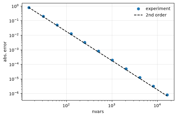
One error value says little. A second-order discretisation should make the error four times smaller whenever the mesh width halves, so we repeat the test of Part A on a sequence of meshes and measure the order.

Along the way, we set up the problem from a parameter dictionary instead of keyword arguments, which is how pySDC is configured from now on.

from collections import namedtuple

import matplotlib.pyplot as plt
import numpy as np

from pySDC.implementations.problem_classes.HeatEquation_ND_FD import heatNd_unforced

problem_params = {
    'nu': 0.1,  # diffusion coefficient
    'freq': 4,  # frequency for the test value
    'bc': 'dirichlet-zero',  # boundary conditions
}

# create list of nvars to do the accuracy test with
nvars_list = [2**p - 1 for p in range(4, 15)]
print(nvars_list)

[15, 31, 63, 127, 255, 511, 1023, 2047, 4095, 8191, 16383]

Collecting results

We store each error in a dictionary, keyed by an ID that says which run it belongs to, and keep the list of nvars in the dictionary too. That makes the results self-describing: the functions that analyse them later need nothing else. The pattern pays off once there are several parameters to vary.

# setup id for gathering the results (will sort by nvars)
ID = namedtuple('ID', 'nvars')


def run_accuracy_check(nvars_list, problem_params):
    """
    Routine to check the error of the Laplacian vs. its FD discretization

    Args:
        nvars_list: list of nvars to do the testing with
        problem_params: dictionary containing the problem-dependent parameters

    Returns:
        a dictionary containing the errors and a header (with nvars_list)
    """

    results = {}
    # loop over all nvars
    for nvars in nvars_list:
        # setup problem
        problem_params['nvars'] = nvars
        prob = heatNd_unforced(**problem_params)

        # create x values, use only inner points
        xvalues = np.array([(i + 1) * prob.dx for i in range(prob.nvars[0])])

        # create a mesh instance and fill it with a sine wave
        u = prob.u_exact(t=0)

        # create a mesh instance and fill it with the Laplacian of the sine wave
        u_lap = prob.dtype_u(init=prob.init)
        u_lap[:] = -((np.pi * prob.freq[0]) ** 2) * prob.nu * np.sin(np.pi * prob.freq[0] * xvalues)

        # compare analytic and computed solution using the eval_f routine of the problem class
        err = abs(prob.eval_f(u, 0) - u_lap)

        # get id for this nvars and put error into dictionary
        id = ID(nvars=nvars)
        results[id] = err

    # add nvars_list to dictionary for easier access later on
    results['nvars_list'] = nvars_list

    return results


results = run_accuracy_check(nvars_list=nvars_list, problem_params=problem_params)

Measuring the order

For two consecutive meshes with \(N_{i-1}\) and \(N_i\) unknowns and errors \(e_{i-1}\), \(e_i\), the observed order is

\[ p_i = \frac{\log(e_{i-1} / e_i)}{\log(N_i / N_{i-1})} . \]

def get_accuracy_order(results):
    """
    Routine to compute the order of accuracy in space

    Args:
        results: the dictionary containing the errors

    Returns:
        the list of orders
    """

    # retrieve the list of nvars from results
    assert 'nvars_list' in results, 'ERROR: expecting the list of nvars in the results dictionary'
    nvars_list = sorted(results['nvars_list'])

    order = []
    # loop over two consecutive errors/nvars pairs
    for i in range(1, len(nvars_list)):
        # get ids
        id = ID(nvars=nvars_list[i])
        id_prev = ID(nvars=nvars_list[i - 1])

        # compute order as log(prev_error/this_error)/log(this_nvars/old_nvars) <-- depends on the sorting of the list!
        tmp = np.log(results[id_prev] / results[id]) / np.log(nvars_list[i] / nvars_list[i - 1])
        order.append(tmp)

    return order


order = get_accuracy_order(results)
for nvars, p in zip(nvars_list[1:], order, strict=True):
    print(f'nvars = {nvars:5d}: computed order {p:4.3f} (expected 2)')

nvars =    31: computed order 1.888 (expected 2)
nvars =    63: computed order 1.949 (expected 2)
nvars =   127: computed order 1.976 (expected 2)
nvars =   255: computed order 1.988 (expected 2)
nvars =   511: computed order 1.994 (expected 2)
nvars =  1023: computed order 1.997 (expected 2)
nvars =  2047: computed order 1.999 (expected 2)
nvars =  4095: computed order 1.999 (expected 2)
nvars =  8191: computed order 1.999 (expected 2)
nvars = 16383: computed order 1.982 (expected 2)

The numbers hover around 2. On a log-log plot, second order is a line with slope \(-2\):

Show code cell source

Hide code cell source

errors = [results[ID(nvars=n)] for n in nvars_list]
fig, ax = plt.subplots(figsize=(6, 4))
ax.loglog(nvars_list, errors, 'o', label='experiment')
ax.loglog(nvars_list, [errors[0] * (nvars_list[0] / n) ** 2 for n in nvars_list], 'k--', label='2nd order')
ax.set_xlabel('nvars')
ax.set_ylabel('abs. error')
ax.grid(alpha=0.3)
ax.legend(frameon=False)
fig.tight_layout()

Warning

Test your operators with care: push nvars beyond \(2^{15}\) and the error grows again. The truncation error is then smaller than the round-off error of the stencil, which divides by \(h^2\).

Try it yourself

Replace the finite-difference stencil by a fourth-order one with problem_params['order'] = 4. Which order do you measure now, and from which nvars on does round-off take over?

Answer

Fourth order (4.1 to 4.9 on the coarse meshes, then 3.99), but only up to 2047 unknowns, where the error bottoms out near \(10^{-9}\); from 4095 on it grows again. That is much earlier than with the second-order stencil, because the error is so much smaller. The check in the last cell then fails, of course: it expects second order.

Summary

• Collect results in a dictionary with IDs for the runs and a header with the metadata.

• Measure orders of accuracy, don’t eyeball them.

The check the tests run:

assert all(np.isclose(order, 2, rtol=0.06)), f"ERROR: spatial order of accuracy is not as expected, got {order}"