Part A: Spatial problem setup

We start as simple as possible: no SDC, no time stepping, just a spatial problem. pySDC calls this a problem class: it holds the spatial discretisation of an equation and knows how to evaluate its right-hand side. Here we take heatNd_unforced, the heat equation

\[ u_t = \nu\, \Delta u \quad \text{on } [0, 1], \qquad u(0, t) = u(1, t) = 0, \]

discretised with second-order finite differences.

import numpy as np
import matplotlib.pyplot as plt

from pySDC.implementations.problem_classes.HeatEquation_ND_FD import heatNd_unforced

prob = heatNd_unforced(
    nvars=1023,  # number of degrees of freedom
    nu=0.1,  # diffusion coefficient
    freq=4,  # frequency of the test function
    bc='dirichlet-zero',  # boundary conditions
)
print(f'{prob.nvars[0]} unknowns, mesh width {prob.dx:.2e}, operator of shape {prob.A.shape}')

1023 unknowns, mesh width 9.77e-04, operator of shape (1023, 1023)

Parameters go in as keyword arguments. Almost everything in pySDC is configured this way; later, the same arguments are collected in a dictionary and handed over to the controller.

Data types

The values of a solution live in a pySDC data type, here mesh, which is a NumPy array with some extra meta-information. Every problem class says which data type it uses, as dtype_u for the solution and dtype_f for the right-hand side, and every data type is created from the problem’s init attribute:

u = prob.dtype_u(init=prob.init)
print(type(u).__name__, u.shape, 'init =', prob.init)

mesh (1023,) init = (1023, None, dtype('float64'))

Note

init and nvars look the same here, so why two attributes? init is whatever the data type needs to set itself up. For a finite-difference mesh that is just the number of unknowns, but for finite elements it is the function space. So: whenever you create a data type, use init.

Testing the operator

Before building anything on top of this discretisation, we check it. We fill u with \(\sin(\pi k x)\), whose exact right-hand side is \(-\nu (\pi k)^2 \sin(\pi k x)\), and compare that with what eval_f computes. We only use inner points: the boundary values are fixed at zero and are not part of the unknowns.

def run_accuracy_check(prob):
    """
    Routine to check the error of the Laplacian vs. its FD discretization

    Args:
        prob: a problem instance

    Returns:
        the error between the analytic Laplacian and the computed one of a given function
    """

    # create x values, use only inner points
    xvalues = np.array([(i + 1) * prob.dx for i in range(prob.nvars[0])])

    # create a mesh instance and fill it with a sine wave
    u = prob.dtype_u(init=prob.init)
    u[:] = np.sin(np.pi * prob.freq[0] * xvalues)

    # create a mesh instance and fill it with the Laplacian of the sine wave
    u_lap = prob.dtype_u(init=prob.init)
    u_lap[:] = -((np.pi * prob.freq[0]) ** 2) * prob.nu * np.sin(np.pi * prob.freq[0] * xvalues)

    # compare analytic and computed solution using the eval_f routine of the problem class
    err = abs(prob.eval_f(u, 0) - u_lap)

    return err


err = run_accuracy_check(prob)
print(f'Error of the spatial accuracy test: {err:8.6e}')

Error of the spatial accuracy test: 1.981783e-04

abs of a mesh is its maximum norm, so this is the largest pointwise error. Relative to the size of the right-hand side, about \(0.1 \cdot (4\pi)^2 \approx 16\), that is small. Seeing it helps:

Show code cell source

Hide code cell source

x = np.array([(i + 1) * prob.dx for i in range(prob.nvars[0])])
u[:] = np.sin(np.pi * prob.freq[0] * x)
f_exact = -((np.pi * prob.freq[0]) ** 2) * prob.nu * u
f_disc = prob.eval_f(u, 0)

fig, (ax1, ax2) = plt.subplots(1, 2, figsize=(10, 3))
ax1.plot(x, f_exact, lw=3, alpha=0.4, label='exact')
ax1.plot(x, f_disc, '--', label='eval_f')
ax1.set_xlabel('$x$')
ax1.set_title(r'$\nu\,\Delta u$')
ax1.legend(frameon=False)
ax2.plot(x, np.abs(f_disc - f_exact))
ax2.set_xlabel('$x$')
ax2.set_title('pointwise error')
fig.tight_layout()

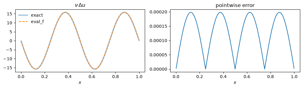
The error has the shape of the solution itself, as expected from the leading term of a second-order finite-difference stencil, \(\frac{h^2}{12} u''''\). In Part B we check that it really shrinks like \(h^2\).

Summary

• A problem class bundles the discretised equation; parameters are passed as keyword arguments.

• Values live in data types such as mesh, created from the problem’s init attribute.

• Test your operators before you build a time integrator on top of them.

The tests check exactly what we saw above:

assert err <= 2e-04, f"ERROR: the spatial accuracy is higher than expected, got {err}"