Part D: Collocation accuracy check

As for space in Part B, we now measure the order of accuracy in time: solve the collocation problem from Part C for a sequence of shrinking time steps and watch the error.

Collocation on \(M\) Gauss-Radau nodes has order \(2M - 1\). We solve a single step, so we see the local error, which is one order higher: \(2M = 6\) for three nodes. Beating sixth order in time with a second-order stencil in space needs a fine mesh, otherwise the spatial error hides everything; hence the 16383 unknowns.

from collections import namedtuple

import matplotlib.pyplot as plt
import numpy as np
import scipy.sparse as sp

from pySDC.core.collocation import CollBase
from pySDC.implementations.problem_classes.HeatEquation_ND_FD import heatNd_unforced

problem_params = {
    'nu': 0.1,  # diffusion coefficient
    'freq': 4,  # frequency for the test value
    'nvars': 16383,  # number of DOFs in space
    'bc': 'dirichlet-zero',  # boundary conditions
}
prob = heatNd_unforced(**problem_params)

# instantiate collocation class, relative to the time interval [0,1]
coll = CollBase(num_nodes=3, tleft=0, tright=1, node_type='LEGENDRE', quad_type='RADAU-RIGHT')

# assemble list of dt
dt_list = [0.1 / 2**p for p in range(0, 5)]

The loop is the one from Part C, once per time step, with the results collected as in Part B.

# setup id for gathering the results (will sort by dt)
ID = namedtuple('ID', 'dt')


def run_accuracy_check(prob, coll, dt_list):
    """
    Routine to build and solve the linear collocation problem

    Args:
        prob: a problem instance
        coll: a collocation instance
        dt_list: list of time-step sizes

    Return:
        the analytic error of the solved collocation problem
    """

    results = {}
    # loop over all nvars
    for dt in dt_list:
        # shrink collocation matrix: first line and column deals with initial value, not needed here
        Q = coll.Qmat[1:, 1:]

        # build system matrix M of collocation problem
        M = sp.eye(prob.nvars[0] * coll.num_nodes) - dt * sp.kron(Q, prob.A)

        # get initial value at t0 = 0
        u0 = prob.u_exact(t=0)
        # fill in u0-vector as right-hand side for the collocation problem
        u0_coll = np.kron(np.ones(coll.num_nodes), u0)
        # get exact solution at Tend = dt
        uend = prob.u_exact(t=dt)

        # solve collocation problem directly
        u_coll = sp.linalg.spsolve(M, u0_coll)

        # compute error
        err = np.linalg.norm(u_coll[-prob.nvars[0] :] - uend, np.inf)
        # get id for this dt and store error in results
        id = ID(dt=dt)
        results[id] = err

    # add list of dt to results for easier access
    results['dt_list'] = dt_list
    return results


def get_accuracy_order(results):
    """
    Routine to compute the order of accuracy in time

    Args:
        results: the dictionary containing the errors

    Returns:
        the list of orders
    """

    # retrieve the list of dt from results
    assert 'dt_list' in results, 'ERROR: expecting the list of dt in the results dictionary'
    dt_list = sorted(results['dt_list'], reverse=True)

    order = []
    # loop over two consecutive errors/dt pairs
    for i in range(1, len(dt_list)):
        # get ids
        id = ID(dt=dt_list[i])
        id_prev = ID(dt=dt_list[i - 1])

        # compute order as log(prev_error/this_error)/log(this_dt/old_dt) <-- depends on the sorting of the list!
        tmp = np.log(results[id] / results[id_prev]) / np.log(dt_list[i] / dt_list[i - 1])
        order.append(tmp)

    return order


results = run_accuracy_check(prob=prob, coll=coll, dt_list=dt_list)
order = get_accuracy_order(results)

# We solve a single step, so this is the local error, which for a collocation method of order 2M-1 is of order 2M.
expected_order = 2 * coll.num_nodes
for dt, p in zip(dt_list[1:], order, strict=True):
    print(f'dt = {dt:.5f}: computed order {p:4.3f} (expected {expected_order})')

dt = 0.05000: computed order 4.791 (expected 6)
dt = 0.02500: computed order 5.364 (expected 6)
dt = 0.01250: computed order 5.675 (expected 6)
dt = 0.00625: computed order 5.865 (expected 6)

Show code cell source

Hide code cell source

errors = [results[ID(dt=dt)] for dt in dt_list]
fig, ax = plt.subplots(figsize=(6, 4))
ax.loglog(dt_list, errors, 'o', label='experiment')
ax.loglog(
    dt_list,
    [errors[-1] * (dt / dt_list[-1]) ** expected_order for dt in dt_list],
    'k--',
    label=f'{expected_order}th order',
)
ax.set_xlabel(r'$\Delta t$')
ax.set_ylabel('abs. error')
ax.grid(alpha=0.3)
ax.legend(frameon=False)
fig.tight_layout()

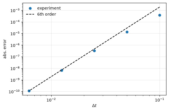
The orders approach 6 from below. The large time steps are not in the asymptotic regime yet: for the largest, \(|\lambda \Delta t| = \nu (4\pi)^2 \Delta t \approx 1.6\) for the sine we start from. This test is also less clean than the spatial one because the error we are after is tiny: we are computing a solution that decays towards zero, very, very thoroughly.

Try it yourself

Switch to quad_type='LOBATTO'. Both ends of the interval are nodes now, so the last node is still the end point and nothing else has to change. Which order do you get?

Answer

About 4.9 for the smallest step, approaching 5: Gauss-Lobatto collocation with \(M\) nodes has order \(2M - 2\), so the local error is of order \(2M - 1 = 5\). The check in the last cell therefore fails: it only looks at the last, asymptotic value and demands it to be close to 6, which is exactly what tells the two node types apart.

Summary

• Collocation on \(M\) Radau nodes is a method of order \(2M - 1\); one step shows the local order \(2M\).

• Measuring temporal orders needs a spatial error well below the temporal one.

This concludes Step 1. In Step 2, we stop solving the collocation problem directly and let SDC do it.

The check the tests run:

assert np.isclose(order[-1], expected_order, atol=0.3), f"ERROR: did not get order of accuracy as expected, got {order}"