

Part D: Writing solutions to file#
The statistics of Parts A to C live in memory, which is fine for a few numbers per step. The solution of a PDE on
a fine grid, recorded for a long run, is better written to disk. pySDC has a hook for that: LogToFile writes the
solution at regular intervals to a single binary file, using the file handlers of
pySDC.helpers.fieldsIO. The same file can be read back for analysis, or to restart a run where it
stopped.
The problem class decides what goes into the file, with two methods: getOutputFile creates the file and writes
its header, and processSolutionForOutput turns a solution into the array that is stored. The problems that
implement them are testequation0d and those built on GenericSpectralLinear, such as the heat, Burgers and
Rayleigh-Bénard equations.
A heat equation#
We take Heat2DChebychev, the heat equation on a grid that is periodic in \(x\) and has Dirichlet boundaries in
\(y\). The boundary values are \(0\) at the bottom and \(1\) at the top, so a sine mode decays towards the linear
profile in between. The problem is written in first-order form, with the derivatives \(u_x\) and \(u_y\) as extra
components, which makes three variables per grid point.
import matplotlib.pyplot as plt
import numpy as np
from pathlib import Path

from pySDC.helpers.fieldsIO import FieldsIO
from pySDC.implementations.controller_classes.controller_nonMPI import controller_nonMPI
from pySDC.implementations.hooks.log_solution import LogToFile
from pySDC.implementations.problem_classes.HeatEquation_Chebychev import Heat2DChebychev
from pySDC.implementations.sweeper_classes.generic_implicit import generic_implicit

# initialize level parameters
level_params = {'restol': 1e-10, 'dt': 0.05}

# initialize sweeper parameters
sweeper_params = {'quad_type': 'RADAU-RIGHT', 'num_nodes': 3, 'QI': 'LU'}

# initialize problem parameters: 32 x 33 points, u = 0 at the bottom and u = 1 at the top
problem_params = {'nx': 32, 'ny': 33, 'a': 0, 'b': 0, 'c': 1, 'nu': 0.1}

# initialize step parameters
step_params = {'maxiter': 20}

# Fill description dictionary for easy hierarchy creation
description = {
    'problem_class': Heat2DChebychev,
    'problem_params': problem_params,
    'sweeper_class': generic_implicit,
    'sweeper_params': sweeper_params,
    'level_params': level_params,
    'step_params': step_params,
}

Path("data").mkdir(parents=True, exist_ok=True)
Configuring the hook#
LogToFile is configured with class attributes. We set them on a subclass of our own, so that other runs in the
same Python process keep the defaults:
filename: the file to write,time_increment: the time between two solutions in the file, here two steps,allow_overwriting: whether an existing file may be replaced. We allow it, so that this page can run again.
Besides the solutions every time_increment, the hook writes the initial conditions and the solution at the end.
class MyLogToFile(LogToFile):
    filename = 'data/step_3_D_heat.pysdc'
    time_increment = 0.1
    allow_overwriting = True


# initialize controller parameters
controller_params = {
    'hook_class': MyLogToFile,
    'logger_level': 30,  # reduce verbosity, the hook tells what it writes on level 20
}
We run up to \(t=0.5\) for now:
controller = controller_nonMPI(num_procs=1, controller_params=controller_params, description=description)
P = controller.MS[0].levels[0].prob
uend, stats = controller.run(u0=P.u_exact(0), t0=0.0, Tend=0.5)
Reading the file#
FieldsIO.fromFile reads any file written this way. From the header it finds out what kind of file it is (here a
Rectilinear grid) and returns the matching handler:
file = FieldsIO.fromFile(MyLogToFile.filename)
print(file)
print('variables:', file.nVar, ' grid:', file.gridSizes)
print('times:', np.round(file.times, 12))
FieldsIO[Rectilinear|float64|file:data/step_3_D_heat.pysdc]<0x7f5329d9c050>
variables: 3  grid: [32, 33]
times: [0.  0.1 0.2 0.3 0.4 0.5]
readField returns the time and the solution at an index in the file. The solution has one array per variable,
on the grid whose coordinates are stored in the header:
t, u = file.readField(-1)
print(f't = {t:.2f}, u has shape {u.shape}')
x, y = file.header['coords']
print(f'x from {x.min():.2f} to {x.max():.2f}, y from {y.min():.2f} to {y.max():.2f}')
t = 0.50, u has shape (3, 32, 33)
x from 0.00 to 6.09, y from -1.00 to 1.00
Restarting from the file#
Now we carry on to \(t=1\). A new run that starts at \(t_0 > 0\) appends to an existing file instead of replacing it,
whatever allow_overwriting says. load gets the solution at an index of the file back. What was written is the
output of processSolutionForOutput, the real solution on the grid, which is what this problem computes with anyway,
so it can go straight into a new initial condition:
restart = MyLogToFile.load(-1)
u0 = P.u_init
u0[:] = restart['u']

controller = controller_nonMPI(num_procs=1, controller_params=controller_params, description=description)
uend, stats = controller.run(u0=u0, t0=restart['t'], Tend=1.0)

file = FieldsIO.fromFile(MyLogToFile.filename)
print('times:', np.round(file.times, 12))
times: [0. 0.1 0.2 0.3 0.4 0.5 0.6 0.7 0.8 0.9 1. ]
The file now holds the whole run. Here is \(u\), the first variable, at three of its times:
<matplotlib.colorbar.Colorbar at 0x7f531c9116a0>
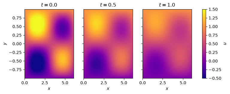
The sine mode decays and leaves the linear profile between the boundaries. For this problem the exact solution is known, so we can check the last solution in the file:
t, u = file.readField(-1)
err = np.max(np.abs(u[0] - P.u_exact(t)[0]))
print(f'error at t={t:.1f}: {err:.3e}')
error at t=1.0: 2.373e-11
The file format#
A file starts with a header: the kind of file and the data type of the values, then, for a Rectilinear grid, the
number of variables, the dimension, the number of points and the coordinates in each direction. After that come
the solutions, each one a time followed by the values of all variables on the whole grid. As each solution takes
the same number of bytes, readField jumps straight to the one it needs, and appending is cheap.
The handlers are not tied to pySDC’s controller. pySDC.helpers.fieldsIO shows how to write and read a
file by hand, and Rectilinear.toVTR converts the solutions of a 3D grid into VTR files for ParaView.
With MPI#
When the problem is distributed over several processes in space, all of them write into the same file, each its
own part of the grid, with collective MPI-IO. The problem sets this up in setUpFieldsIO, which tells
Rectilinear.setupMPI the part of the grid of each process. The header always holds the global grid, so a file
written by any number of processes can be read by any other number, in serial as well. The spectral problems do all
this by themselves, and the hook is used exactly as above.
Important things to note
Configure
LogToFilewith class attributes on a subclass, so that other runs keep the defaults.Without
allow_overwriting, the hook will neither replace an existing file nor write a solution at a time the file already has.To write another problem to file, implement
getOutputFileandprocessSolutionForOutputin its class, and, for MPI,setUpFieldsIO.
The checks the tests run:
assert np.allclose(file.times, np.arange(11) * 0.1), f'ERROR: unexpected times in the file: {file.times}'
assert err < 1e-8, f'ERROR: solution is not as exact as expected, got {err}'