

Part D: MLSDC with particles#
Back to the Boris solver and the Penning trap of Step 3, now with 50 particles,
to show that coarsening can go beyond the number of unknowns or collocation nodes. The costly part of this
problem is the force: every particle interacts with every other one, \(O(N^2)\) work. On the coarse level, we use
a simpler problem, penningtrap_coarse in PenningTrap_3D_coarse.py next to this tutorial, which leaves out the
particle-particle interaction and only computes the external fields, \(O(N)\) work. For this, the problem class in
the description simply becomes a list of two classes.
The transfer class particles_to_particles is a dummy: both levels have the same particles, so there is nothing
to restrict or interpolate but the values themselves.
import importlib.util
import time

import matplotlib.pyplot as plt
import numpy as np

from pySDC.helpers.stats_helper import get_sorted
from pySDC.implementations.controller_classes.controller_nonMPI import controller_nonMPI
from pySDC.implementations.problem_classes.PenningTrap_3D import penningtrap
from pySDC.implementations.sweeper_classes.boris_2nd_order import boris_2nd_order
from pySDC.implementations.transfer_classes.TransferParticles_NoCoarse import particles_to_particles
from pySDC.tutorial.step_3.HookClass_Particles import particle_hook
from pySDC.tutorial.step_4.PenningTrap_3D_coarse import penningtrap_coarse


def run_penning_trap_simulation(mlsdc, finter=False):
    """
    Run one step of the Penning trap with SDC or MLSDC, and return the statistics, the run time and the number of
    right-hand side evaluations on each level
    """
    # initialize level parameters
    level_params = {'restol': 1e-07, 'dt': 1.0 / 8}

    # initialize sweeper parameters
    sweeper_params = {'quad_type': 'RADAU-RIGHT', 'num_nodes': 5}

    # initialize problem parameters for the Penning trap
    problem_params = {
        'omega_E': 4.9,  # E-field frequency
        'omega_B': 25.0,  # B-field frequency
        'u0': np.array([[10, 0, 0], [100, 0, 100], [1], [1]], dtype=object),  # initial center of positions
        'nparts': 50,  # number of particles in the trap
        'sig': 0.1,  # smoothing parameter for the forces
    }

    # initialize step parameters
    step_params = {'maxiter': 20}

    # initialize controller parameters
    controller_params = {
        'hook_class': particle_hook,  # specialized hook class for more statistics and output
        'logger_level': 30,
    }

    transfer_params = {'finter': finter}

    # Fill description dictionary for easy hierarchy creation
    description = {
        # MLSDC: a list of two problem classes, one for the fine and one for the coarse level
        'problem_class': [penningtrap, penningtrap_coarse] if mlsdc else penningtrap,
        'problem_params': problem_params,
        'sweeper_class': boris_2nd_order,
        'sweeper_params': sweeper_params,
        'level_params': level_params,
        'step_params': step_params,
        'space_transfer_class': particles_to_particles,
        'base_transfer_params': transfer_params,
    }

    # instantiate the controller
    controller = controller_nonMPI(num_procs=1, controller_params=controller_params, description=description)

    # set time parameters
    t0 = 0.0
    Tend = level_params['dt']

    # get initial values on finest level
    P = controller.MS[0].levels[0].prob
    uinit = P.u_init()

    # call and time main function to get things done...
    start_time = time.perf_counter()
    uend, stats = controller.run(u0=uinit, t0=t0, Tend=Tend)
    end_time = time.perf_counter() - start_time

    rhs = [L.prob.work_counters['rhs'].niter for L in controller.MS[0].levels]
    return stats, end_time, rhs
Three runs#
SDC, MLSDC, and MLSDC with interpolation of the right-hand side (finter, see
Part C). Where numba is available, it compiles the force computation the first time it is
called; a run beforehand keeps that out of the timings.
if importlib.util.find_spec('numba') is not None:
    run_penning_trap_simulation(mlsdc=False)  # compiles the force computation

# run SDC, MLSDC and MLSDC plus f-interpolation and compare
stats_sdc, time_sdc, rhs_sdc = run_penning_trap_simulation(mlsdc=False)
stats_mlsdc, time_mlsdc, rhs_mlsdc = run_penning_trap_simulation(mlsdc=True)
stats_mlsdc_finter, time_mlsdc_finter, rhs_mlsdc_finter = run_penning_trap_simulation(mlsdc=True, finter=True)

runs = {
    'SDC': (stats_sdc, time_sdc, rhs_sdc),
    'MLSDC': (stats_mlsdc, time_mlsdc, rhs_mlsdc),
    'MLSDC+finter': (stats_mlsdc_finter, time_mlsdc_finter, rhs_mlsdc_finter),
}
for name, (stats, runtime, rhs) in runs.items():
    niter = get_sorted(stats, type='niter')[0][1]
    print(f'{name:13s}: {niter:2d} iterations, {runtime:6.3f} s, right-hand side evaluations per level {rhs}')
step - WARNING: you have specified transfer classes, but only a single level
step - WARNING: you have specified transfer classes, but only a single level
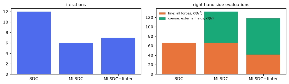
SDC          : 12 iterations,  1.678 s, right-hand side evaluations per level [66]
MLSDC        :  6 iterations,  1.873 s, right-hand side evaluations per level [66, 66]
MLSDC+finter :  7 iterations,  2.091 s, right-hand side evaluations per level [41, 77]
Energy#
All three produce more or less the same energy:
# sort and convert stats to list, sorted by iteration numbers (only pre- and after-step are present here)
energy_sdc = get_sorted(stats_sdc, type='etot', sortby='iter')
energy_mlsdc = get_sorted(stats_mlsdc, type='etot', sortby='iter')
energy_mlsdc_finter = get_sorted(stats_mlsdc_finter, type='etot', sortby='iter')

# get base energy and show differences
base_energy = energy_sdc[0][1]
for energy in [energy_sdc, energy_mlsdc, energy_mlsdc_finter]:
    for item in energy:
        print(
            'Total energy and relative deviation in iteration %2i: %12.10f -- %12.8e'
            % (item[0], item[1], abs(base_energy - item[1]) / base_energy)
        )
Total energy and relative deviation in iteration  0: 407936.7556966486 -- 0.00000000e+00
Total energy and relative deviation in iteration 12: 406977.9425667248 -- 2.35039652e-03
Total energy and relative deviation in iteration  0: 407936.7556966486 -- 0.00000000e+00
Total energy and relative deviation in iteration  6: 406977.9425660007 -- 2.35039652e-03
Total energy and relative deviation in iteration  0: 407936.7556966486 -- 0.00000000e+00
Total energy and relative deviation in iteration  7: 406977.9428639796 -- 2.35039579e-03
Iterations, work and time#
MLSDC takes half as many iterations as SDC, and with finter one more. But look at the expensive evaluations on
the fine level: MLSDC needs as many as SDC, because each interpolation needs the fine right-hand side again, as
we saw in Part C. Only interpolating the right-hand side as well (finter) saves some of them.
Whether that shows in the run times depends on how expensive the fine force really is compared with everything
else in a sweep. With numba, as when this page was built, 50 particles are cheap: SDC tends to be fastest, and
finter costs more than it saves. Without numba the forces weigh more and the gap closes; in our runs, MLSDC with
finter then came out slightly ahead of SDC in plain Python, while in the browser, which has no numba either, all
three were within a few percent. Press Run in browser to see for yourself. Timings depend on
the machine and the implementation; the counts above do not.
Important things to note
Again, the number of MLSDC iterations is highly sensitive to the interplay of all the parameters (number of particles, smoothing parameter, number of nodes, residual tolerance, …). It is by far not trivial to get a speedup at all, although a reasonable setup has been chosen here.
Count the work, not only the iterations: what an iteration costs differs between the methods.
This kind of coarsening can be combined with the generic ones of Part B. Yet, using fewer collocation nodes on the coarse level increases the iteration counts here.
The checks the tests run:
deviation_mlsdc = abs(energy_sdc[-1][1] - energy_mlsdc[-1][1]) / base_energy
deviation_finter = abs(energy_mlsdc[-1][1] - energy_mlsdc_finter[-1][1]) / base_energy
assert deviation_mlsdc < 6e-10, f'ERROR: energy deviated too much between SDC and MLSDC, got {deviation_mlsdc}'
assert deviation_finter < 8e-10, f'ERROR: energy deviated too much after using finter, got {deviation_finter}'