Resilience in SDC
In this project, we try a few methods for fixing bitflips in the solution caused by external factors such as radiation. For convenience, we show here plots of tests which are generated by the continuous integration pipeline on GitHub, meaning they are always generated by the latest master branch, while showing explanations in jupyter notebooks, which show only a fixed commit.
The first strategy we try is Adaptivity, which continually adjusts the step size during run-time and comes with resilience as a by product.
The second strategy is Hot Rod, which is designed purely as a detector for soft faults.
We have also simulated faults in the van der Pol problem and tried recovering them with the strategies here. We also experimented with faults in the Lorenz attractor problem. See Resilience in the Lorenz Attractor.
Tests
Please refer to the above mentioned notebooks for thorough descriptions of what you are seeing here. These plots are duplicates of what you can find there, but generated with the latest master branch.
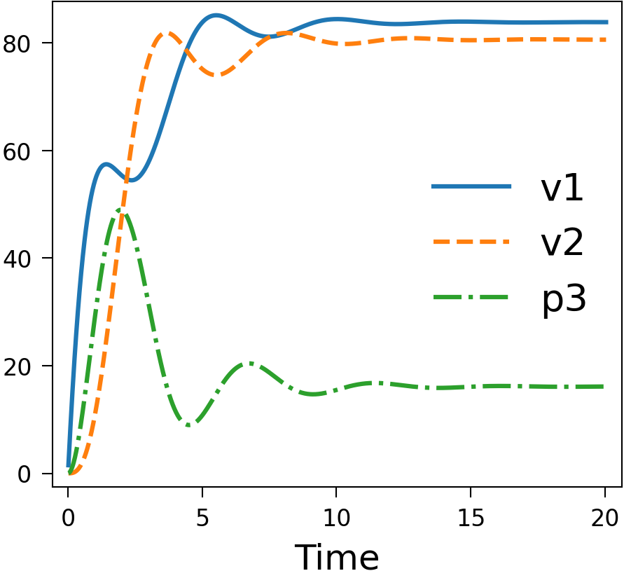
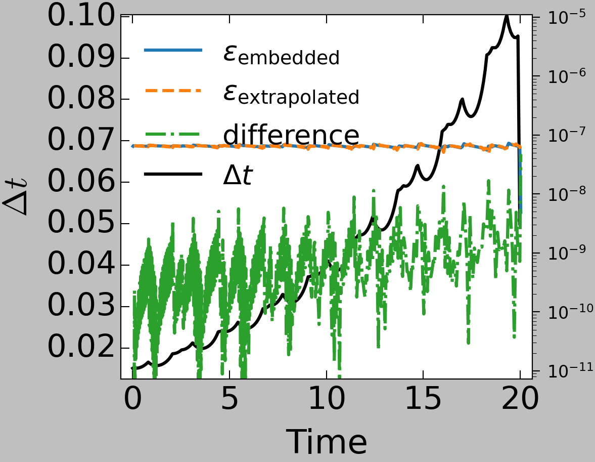
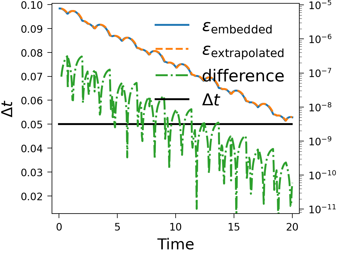
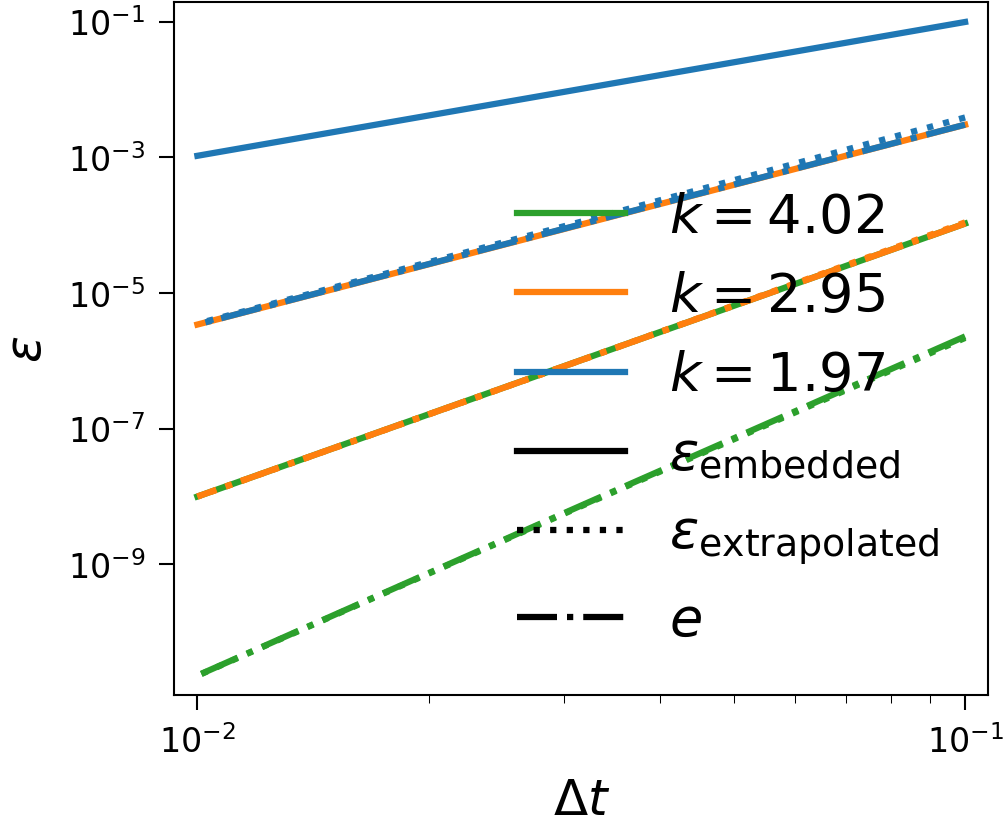
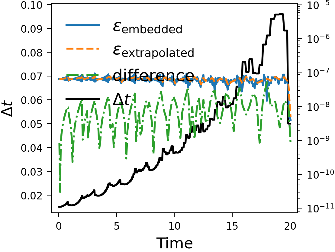
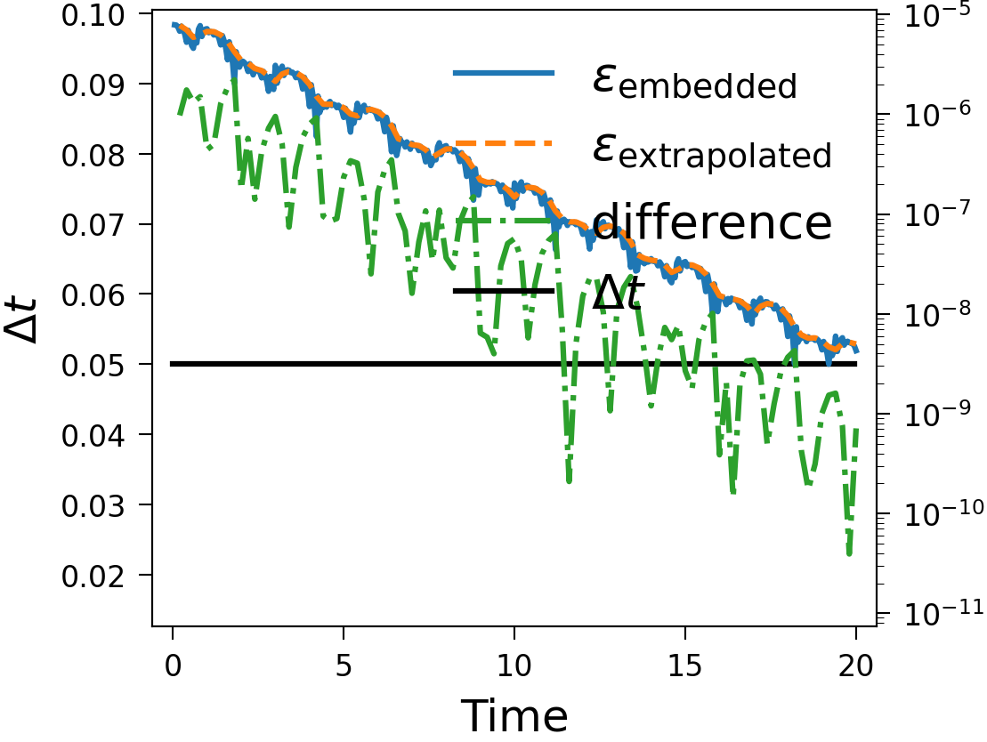
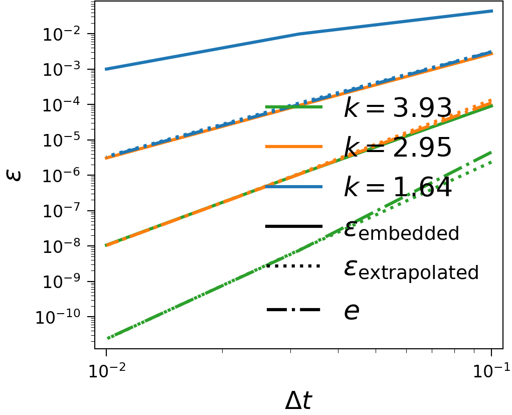
The Piline equation models an electrical start-up process and is a system of ordinary differential equations, that shows some slowing down of the time scale and is hence a good test to check adaptivity with. See below for, in the order of mention, plots of the solution, the error estimates with difference for Hot Rod and time step with adaptivity enabled and the same with fixed time step and the order of the error estimates with different numbers of sweeps. The last plot was made without Hot Rod, meaning the last sweep is taken to be the solution of the time step, making it one order higher than the embedded estimate, and it can be seen that the extrapolation error estimate lies on top of the embedded error estimate with one fewer sweep. These plots were generated with serial SDC.
We also have an implementation for Block Gauss-Seidel multi-step SDC in a simulated parallelism version without MPI. You can see the results below, except for the solution, which looks the same as the serial solution to the naked eye.
Reproduction of the plots in the adaptive SDC paper
To reproduce the plots you need to install pySDC using this project’s environment.yml file, which is in the same directory as this README. Then, run the following commands in the same directory:
mpirun -np 4 python work_precision.py --mode=compare_strategies --problem=vdp
mpirun -np 4 python work_precision.py --mode=compare_strategies --problem=quench
mpirun -np 4 python work_precision.py --mode=compare_strategies --problem=Schroedinger
mpirun -np 4 python work_precision.py --mode=compare_strategies --problem=AC

mpirun -np 12 python work_precision.py --mode=parallel_efficiency --problem=vdp
mpirun -np 12 python work_precision.py --mode=parallel_efficiency --problem=quench
mpirun -np 12 python work_precision.py --mode=parallel_efficiency --problem=Schroedinger
mpirun -np 12 python work_precision.py --mode=parallel_efficiency --problem=AC

mpirun -np 4 python work_precision.py --mode=RK_comp --problem=vdp
mpirun -np 4 python work_precision.py --mode=RK_comp --problem=quench
mpirun -np 4 python work_precision.py --mode=RK_comp --problem=Schroedinger
mpirun -np 4 python work_precision.py --mode=RK_comp --problem=AC

python paper_plots.py --target=adaptivity
Possibly, you need to create some directories in this one to store and load things, if path errors occur.
Reproduction of the plots in the resilience paper
To reproduce the plots you need to install pySDC using this project’s environment.yml file, which is in the same directory as this README. Then, run the following commands in the same directory:
mpirun -np 4 python fault_stats.py prob run_Lorenz
mpirun -np 4 python fault_stats.py prob run_Schroedinger
mpirun -np 4 python fault_stats.py prob run_AC
mpirun -np 4 python fault_stats.py prob run_RBC
python paper_plots.py --target=resilience
Please be aware that generating the fault data for Rayleigh-Benard requires generating reference solutions, which may take several hours.
Reproduction of the plots in Thomas Baumann’s thesis
To reproduce the plots you need to install pySDC using this project’s environment.yml file, which is in the same directory as this README.
To run the resilience experiments, run
mpirun -np 4 python fault_stats.py prob run_Lorenz
mpirun -np 4 python fault_stats.py prob run_vdp
mpirun -np 4 python fault_stats.py prob run_GS
mpirun -np 4 python fault_stats.py prob run_RBC
Please be aware that generating the fault data for Rayleigh-Benard requires generating reference solutions, which may take several hours. To run the experiments on computational efficiency, run for the choices of problems vdp, Lorenz`, GS, RBC the following commands
mpirun -np 4 python work_precision.py --mode=compare_strategies --problem=<problem>
mpirun -np 12 python work_precision.py --mode=parallel_efficiency_dt_k --problem=<problem>
mpirun -np 12 python work_precision.py --mode=parallel_efficiency_dt --problem=<problem>
mpirun -np 12 python work_precision.py --mode=RK_comp --problem=<problem>
After you ran all experiments, you can generate the plots with the following command:
python paper_plots.py --target=thesis
As this plotting script also runs a few additional smaller experiments, do not be surprised if it takes a while.